ELIAS NEMA - 🔮 State of Recommendations

Overview

This is a lengthy piece covering 6 articles, 4 papers and demonstrating trends happening in the field of applied recommender systems. Cases below will be structured as follows:

flowchart LR
  A(Overview) --> B(Data)
  B --> C(Model)
  C --> D(Validation)
  D --> E(Production)

I prefer not to focus on the reported results because they are usually relative to the previous baselines and easily interpreted outside the context.

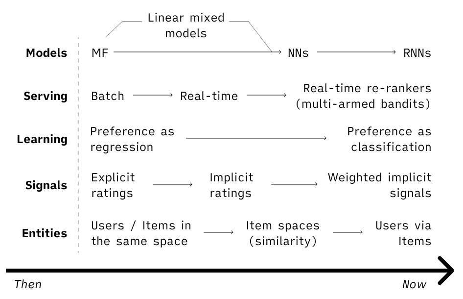
Starting back in the days with a timeless classic of recsys — matrix factorization, it’s now hard to find a system without some kind of neural nets, embedding spaces or sequential models.

Serving has also moved to more real-time architectures and dynamic re-rankers. Not to mention that generally, the focus now is much more on the system as a whole, rather than just a modeling part.

Moving from relying mostly on explicit ratings to incorporating different implicit signals and giving them weights. Hence, also the regression→classification shift.

On the item side pretty much every one converged to building embeddings to optimize for the product similarity.

On the user side, however, representations vary depending on the use case and business model.

But the truth is in details, so let’s dive in.

LinkedIn Learning

We start with the LinkedIn Learning use case and their two-part article (one, two). The main goal for them is to “surface the most relevant and personalized course recommendations”.

At LinkedIn, two main models are powering the offline (precalculated for each user daily) recommendations — neural collaborative filtering and “response prediction” model.

LinkedIn Learning: Collaborative Filtering (Neural)

Pros/cons of CF are well-known and LinkedIn didn’t escape them. Here is their recap:

works better for core learners (members who are already active on the LinkedIn Learning platform)
focuses on recent interactions (not a very common one, probably a property of their implementation)
diversified recommendations, no domain knowledge needed, however, cold start problems

I think recency and diversity are the most interesting points here.

Recency: generally, CF doesn’t give preference for the recent items unless implemented with some kind of time decay or position-aware component in the model.

Diversity: in e-commerce, CF often reduces diversity because of the rich-get-richer effect. And here, probably, due to the fact that the course catalog is not that big and that every person can take any course, it actually increases it.

🛢Data: course watch history data with a watch-time threshold (if a learner only watches the first three seconds of a course, it’s not included).

🚗Model:

Computing learner and course embeddings in parallel. This is also known as a two-tower architecture.
Log loss is used as an optimization function.
The modeling objective is to predict course watches using the past watches.
4 negative samples are taken for each positive one.
Holding the last interaction for each user for a test set — a leave-one-out approach.

Two-tower architecture consists of two networks with fully connected layers in each becoming narrower with each consecutive layer.

🔁Validation: A random sample of 100 items that user didn’t interact with is taken and the one hidden item (user’s last action) is ranked against these 100. Performance is judged by hit ratio and NDCG at 10.

Interesting that input to the learner part is user/course co-occurrence matrix, while input to the course part is course/course similarity matrix.

🎬Production: Generating top K courses for each user based on the similarity between embeddings. Calculating offline and storing in a key-value storage.

LinkedIn Learning: Response Prediction Model

Another offline model to compliment CF is so-called “Response Prediction”. It takes into account user and course metadata as well as user’s actions.

This algorithm typically performs better than CF for members with no/little previous engagement on LinkedIn Learning, as well as for new courses with few prior interactions.

🛢Data:

User profile features (skills, industry, etc.)
Course metadata (difficulty, category, skills)
Historical explicit engagement (clicks, bookmarks, etc.) with the course watch time as an importance weight given to each click instance.

As a result, this importance weight helps to promote courses with higher watch times and creates a model that can optimize for course watches, not just clicks.

🚗Model: a fancy named “Generalized Linear Mixture Model (GLMix)” is used here. In reality, it’s quite a simple (though hard computationally, check the paper) approach to express user’s probability to click via a sum of the three components: a global model, per-learner model, and per-course model.

We are currently working on a model ensemble that can perform personalized blending of Response Prediction and Neural CF models to improve the overall performance on the final recommendation task. Secondly, we also plan to adopt Attention Models into our Neural CF framework for learner profiling, i.e., assigning attention weights to a learner’s course watch history to capture long term and short term interests in a more effective manner.

🔁Validation: AUC for offline validation as well as click/apply rates for the online experiments.

🎬Production: offline two-stage ranking strategy.

storing courses and their features in Lucene, after, using features of users to generate 1000 candidates for each
ranking candidates using full GLMix model

LinkedIn Jobs

In their next article, LinkedIn shared some insights on their jobs recommendations (which can potentially be useful for any job-seeker). For example:

Our analysis demonstrated that the majority of job applicants apply to at least 5 jobs, while the majority of job postings receive at least 10 applicants. This proves to result in enough data to train the personalization models.

Goal: to predict the probability of a positive recruiter action, conditional on a given member applying to a given job.

🛢Data: how to identify if a signal is negative (have someone not replied because of lack of interest or because he is processing other candidates)? > We make the negatives conclusive if no engagement is seen after 14 days. However, if a recruiter responds to other applications submitted later, we may infer the negative label earlier.

Now you know when to stop waiting for the recruiter’s response ⏳.

🚗Model: here, the same model from the above (GLMix).

logit(P(positive response | member, job)) =
F_global(X_member, X_job) + F_member(X_job) + F_job(X_member)

We used linear models for fm and fj, but one can use any model in the above formulation as long as the produced scores are calibrated to output log-odds (for example, a neural net). Usually, linear models are sufficient as per-member and per-job components, as individual members and individual jobs do not have enough interactions to train more complex non-linear models.

🔁Validation: AUC and NDCG are used.

🎬Production:

user/job models are retrained daily, with automated quality checks in place
global model his updated once every few weeks
initializing weights with existing values to reduce the training time

You can see that features of your profile play a very important role when you are searching for a job, so if you are looking for something specific, make sure to include the relevant signals into your profile at least a couple of days before.

Avito

A very important and thoughtful article (in Russian) from our friends at Avito. And their approach takes a bit different direction. What if instead of learning personalized recommendations we’d try to optimize for the item similarity?

🛢Data: pairs of “similar” items.

How to define similars? Items that were “contacted” (the best proxy for the transaction in classifieds) by a user with a time threshold between actions (8h for Avito). This gives 1s as a label. How to get 0s? Negative sampling from the items that were active at the platform during the time of contact but were not selected by the user.

Random sampling with a probability of an item being selected equals to a square root of a number of contacts that this item got (how popular the item was).

🚗Model: item features are fed into the embedding layers with a dropout and 2 linear layers on top. Item IDs are not included into item features to allow for model generalization.

The last layer is tanh to transform the output into the [-1, 1] range and multiply by 128 later to fit into the INT8 to save memory in serving.

Calculating scores for the positive sample and 4000 (the more — the better, constraint of the GPU memory) negative samples for each pair. Taking highest scores from the negatives (top 100 wrongly predicted items) and computing the log-loss.

Learning only from the top 100 wrong predictions allows to save on training time without loosing the accuracy.

🔁Validation: precision at 8 is calculated on a test set. Time-based split, with omitting 6 months of data between training and validation. This is done to see how model will behave after 6 months of not training.

🎬Production: The model is re-trained once per 6 months. This works fine because item IDs are not included into training so new items can be embedded into the space just by their features. So new items get’s represented in a space as soon as they are posted. Embeddings are stored in Sphinx search engine, which allows quite a fast vector search (p99 is under 200ms with 200k rpm, sharded by category).

Recommendations are used on both the item page (item-to-item) and the homefeed (user-to-item), with user-to-item generated from the similar items to the ones that user has seen recently.

And now — Pinterest. Another very thoughtful and pragmatic piece from them.

Here as well, the general idea is to embed users/items into some space. However, having a single vector for user works bad — no matter how good the network is it won’t be able to represent all the clusters of user’s interests. Another approach (the same as Avito takes above) is to represent a user via embeddings of items that he is interested in. But averaging of embeddings works bad for the longer-term user interests (e.g. paintings and shoes average to a salad). The solution?

Run clustering on the user’s actions and take medoids (like centroids, but should be an existing item) from the most important clusters. Find similar items to those medoids.

🛢Data: users’ action pins from the last 90 days.

🚗Model: the main model is quite a simple Ward clustering with the goal to produce different amount of clusters depending on a variety of items in the user’s history. A time decay average is used to assign importance to clusters.

🔁Validation: a very thorough approach to the evaluation process, highly recommend to check out more in the paper.

Cluster user’s actions and rank clusters by importance.
Get 400 closest items to the medoids of the most important clusters.
Calculate relevance: the proportion of observed action pins that have high cosine similarity (≥0.8) with any recommended pin.
And recall: the proportion of action pins that are found in the recommendation set.
Test batches are calculated in the chronological order, day by day, simulating the production setup.

🎬Production:

Using HNSW for the approximate nearest neighbor search
Filtering out near-duplicates and lower quality pins
Using medoids allows saving on caching (no need to compute aNN all the time)

Served using a classical lambda architecture:

Daily Batch Inference: PinnerSage is run daily over the last 90 day actions of a user on a MapReduce cluster. The output of the daily inference job (list of medoids and their importance) are served online in key-value store.

Lightweight Online Inference: We collect the most recent 20 actions of each user on the latest day (after the last update to the entry in the key-value store) for online inference. PinnerSage uses a real-time event-based streaming service to consume action events and update the clusters initiated from the key-value store.

In practice, the system optimization plays a critical role in enabling the productionization of PinnerSage.

Coveo

Ok, item embeddings are great. But how about transfer learning for them? Wait, what? The thing is that many companies are actually multi-brand groups having more than one website.

Training embeddings for similar products in different shops will produce spaces which are not comparable. Is there a way to mitigate this? You bet there is.

🛢Data: the best part is that you don’t need tons of data. All you need is data on how users interacted with products within sessions to build product spaces. After that, product features will come handy (text attributes, prices, images, etc.) to align spaces. Having cross-shop data is valuable later but not strictly necessary.

🚗Model: product embeddings are trained using CBOW with negative sampling, by swapping the concept of words in a sentence with products in a browsing session. This is not the fanciest architecture for item embeddings — check the Avito implementation above for a more sophisticated approach.

More interestingly though is a task to align product spaces. It’s different from aligning spaces for languages, mainly, because languanes are guaranteed to have similiar concepts, while for some products it’s not necesseraly true. Coveo has tried different models, but the general approach is:

Start with some unsupervised approach, such as pairing by item features, images, etc. This helps finding the initial mapping function.
Later, adjust the space alignment by learning from user interactions with the items in different spaces.

🔁Validation: for the product embeddings model evaluation is done using the leave-one-out approach and by predicting the Nth interactions from the 0..N-1 items: embeddings are averaged for 0..N-1 items and the nearest neighbor search is done to predict the Nth item. NDCG@10 is used on the search result.

Worth noting that this approach works for the short-lived sessions or specialized shops, while for sessions with multiple intents averaging might produce really weird results (see the Pinterest case above).

🎬Production: they run 2 experiments. In both, the idea was to use an intent from one shop and aligned embeddings to

predict the user’s next action
predict the best query in the search autocomplete

Both experiments have proven the potential behind the approach and I’ll be paying a close attention to the area of transfer learning for product spaces in the future.

References:

LinkedIn’s Learning Recommendations Part 1
LinkedIn’s Learning Recommendations Part 2
LinkedIn’s Neural Collaborative Filtering
LinkedIn’s Generalized Linear Mixed Models
LinkedIn Jobs’ article
Avito’s article
Pinterest’s article
Pinterest’s paper
Coveo’s blog posts: one, two
Coveo’s paper
Intro to recommendations by Google