Introduction
I’ve always wanted to try the makeover monday since I learned about the project. But busy being busy , you know.
Last week, however, two things happened:
Arsenal’s last season stats were posted as a weekly project (and I love football).
I accidentally noticed that.
So it was decided - I’m creating a visualisation.
Code
# Imports import pandas as pdimport plotly.express as px% matplotlib inlineimport matplotlib.pyplot as pltfrom pandas.plotting import scatter_matriximport plotly.io as pio= "notebook" import warnings= 'ignore' )'display.max_columns' , None )= pd.read_excel('Arsenal Player Stats 2018-19.xlsx' )
EDA
Code
print (f'columns: { df. columns} ' )
columns: Index(['Rank', 'Player', 'Nationality', 'Metric', 'Stat'], dtype='object')
Code
0
1
Pierre-Emerick Aubameyang
Gabon
Appearances
36
1
2
Alex Iwobi
Nigeria
Appearances
35
2
2
Alexandre Lacazette
France
Appearances
35
3
4
Lucas Torreira
Uruguay
Appearances
34
4
5
Matteo Guendouzi
France
Appearances
33
You can see that data is stored as rows per player/metric pair. Let’s pivot to get the player’s statistics in each row.
Code
= df.pivot(index= 'Player' , columns= 'Metric' , values= 'Stat' )
Player
Aaron Ramsey
28
6
2
3
0
27
21
4
0
0
1328
4
0
773
0
0
0
33
34
1029
0
Ainsley Maitland-Niles
16
1
0
11
1
17
8
1
0
0
986
1
0
451
0
1
0
5
33
782
1
Alex Iwobi
35
6
3
10
0
56
8
3
0
0
1972
2
0
951
0
0
0
35
28
1415
0
Alexandre Lacazette
35
8
13
29
0
61
51
13
0
1
2505
24
0
771
0
0
0
81
35
1313
2
Bernd Leno
32
0
0
32
0
1
0
0
10
0
2835
0
0
922
16
0
105
0
0
1276
0
Adding Positions
I wanted to cluster players together to see if there are any patterns and groups. Then realised - it doesn’t make a good visualisation: hey, look, these players have more Saves - they are probably goalkeepers. So I decided to add player field position to the dataset.
With this data, let’s look at performance by position. Maybe a radar chart can work for such kind of comparison?
There is a limited amount of axes on a graph for users to still make sense of it. How to choose metrics to display? There are obvious choices of course: saves for goalkeepers, tackles for defenders, goals for forwards . But how about common attributes such as passes or touches ?
To identify potentially interesting data points, I started with a correlation plot. I’m looking for interesting patterns, i.e. metrics that are not linearly correlated with the minutes played.
Code
= {k:'' for k in training.index.tolist()}for gk in ['Bernd Leno' , 'Petr Cech' ]:= 'GK' for df in ['Carl Jenkinson' ,'Héctor Bellerín' ,'Laurent Koscielny' ,'Rob Holding' ,'Sead Kolasinac' 'Shkodran Mustafi' ,'Sokratis' ,'Stephan Lichtsteiner' = 'DF' for mf in ['Aaron Ramsey' ,'Ainsley Maitland-Niles' ,'Denis Suárez' ,'Granit Xhaka' ,'Henrikh Mkhitaryan' 'Joe Willock' ,'Konstantinos Mavropanos' ,'Lucas Torreira' , 'Matteo Guendouzi' ,'Mesut Özil' 'Mohamed Elneny' ,'Nacho Monreal' ,= 'MF' for fw in ['Alex Iwobi' ,'Alexandre Lacazette' ,'Bukayo Saka' ,'Danny Welbeck' ,'Eddie Nketiah' ,'Pierre-Emerick Aubameyang' = 'FW' 'position' ] = training.index.map (position_lookup)
Code
= training.groupby('position' ).sum ()
position
DF
143
12
2
459
1
64
143
6
0
0
11479
17
1
6968
0
0
0
64
201
9185
34
FW
120
20
39
59
0
156
76
40
0
5
7425
51
0
2488
0
0
0
217
88
3984
2
GK
39
0
0
39
0
1
0
0
16
0
3420
0
0
1146
18
0
133
0
1
1591
0
MF
229
20
9
205
2
188
193
23
0
3
15241
21
0
10203
0
2
0
186
319
13366
36
Code
# Common metrics 'passes_per_min_played' ] = training['Passes' ] / training['Minutes Played' ]'passes_per_appearance' ] = training['Passes' ] / training['Appearances' ]'min_played_per_apperance' ] = training['Minutes Played' ] / training['Appearances' ]'touches_per_appearance' ] = training['Touches' ] / training['Appearances' ]'touches_per_min_played' ] = training['Touches' ] / training['Minutes Played' ]# GK metrics 'high_claim_per_min_played' ] = training['High Claim' ] / training['Minutes Played' ]'punches_per_min_played' ] = training['Punches' ] / training['Minutes Played' ]'saves_per_min_played' ] = training['Saves' ] / training['Minutes Played' ]'high_claim_per_appearance' ] = training['High Claim' ] / training['Appearances' ]'punches_per_appearance' ] = training['Punches' ] / training['Appearances' ]'saves_per_appearance' ] = training['Saves' ] / training['Appearances' ]# DF metrics 'clearances_per_min_played' ] = training['Clearances' ] / training['Minutes Played' ]'clearances_per_appearance' ] = training['Clearances' ] / training['Appearances' ]'clearances_per_touch' ] = training['Clearances' ] / training['Touches' ]'fouls_per_appearance' ] = training['Fouls' ] / training['Appearances' ]'fouls_per_clearance' ] = training['Fouls' ] / training['Clearances' ]'fouls_per_touch' ] = training['Fouls' ] / training['Touches' ]'yc_per_min_played' ] = training['Yellow Cards' ] / training['Minutes Played' ]'yc_per_tackle' ] = training['Yellow Cards' ] / training['Tackles' ]'yc_per_foul' ] = training['Yellow Cards' ] / training['Fouls' ]'tackles_per_appearance' ] = training['Tackles' ] / training['Appearances' ]'tackles_per_min_played' ] = training['Tackles' ] / training['Minutes Played' ]# Midfield metrics 'assists_per_appearance' ] = training['Assists' ] / training['Appearances' ]'assists_per_min_played' ] = training['Assists' ] / training['Minutes Played' ]'assists_per_pass' ] = training['Assists' ] / training['Passes' ]'assists_per_touch' ] = training['Assists' ] / training['Touches' ]'dispossessed_per_appearance' ] = training['Dispossessed' ] / training['Appearances' ]'dispossessed_per_min_played' ] = training['Dispossessed' ] / training['Minutes Played' ]'dispossessed_per_pass' ] = training['Dispossessed' ] / training['Passes' ]'dispossessed_per_touch' ] = training['Dispossessed' ] / training['Touches' ]'fouls_per_appearance' ] = training['Fouls' ] / training['Appearances' ]'fouls_per_clearance' ] = training['Fouls' ] / training['Clearances' ]'fouls_per_min_played' ] = training['Fouls' ] / training['Minutes Played' ]'fouls_per_touch' ] = training['Fouls' ] / training['Touches' ]'goals_per_appearance' ] = training['Goals' ] / training['Appearances' ]'goals_per_min_played' ] = training['Goals' ] / training['Minutes Played' ]'goals_per_shot' ] = training['Goals' ] / training['Shots' ]'goals_per_touch' ] = training['Goals' ] / training['Touches' ]'passes_per_appearance' ] = training['Passes' ] / training['Appearances' ]'passes_per_min_played' ] = training['Passes' ] / training['Minutes Played' ]'passes_per_touches' ] = training['Passes' ] / training['Touches' ]'shots_per_appearance' ] = training['Shots' ] / training['Appearances' ]'shots_per_min_played' ] = training['Shots' ] / training['Minutes Played' ]'shots_per_touch' ] = training['Shots' ] / training['Touches' ]'tackles_per_appearance' ] = training['Tackles' ] / training['Appearances' ]'tackles_per_min_played' ] = training['Tackles' ] / training['Minutes Played' ]'tackles_per_touch' ] = training['Tackles' ] / training['Touches' ]'tackles_per_clearance' ] = training['Tackles' ] / training['Clearances' ]'touches_per_apperance' ] = training['Touches' ] / training['Appearances' ]'touches_per_min_played' ] = training['Touches' ] / training['Minutes Played' ]# FW metrics 'assists_per_min_played' ] = training['Assists' ] / training['Minutes Played' ]'missed_chances_per_shot' ] = training['Big Chances Missed' ] / training['Shots' ]'missed_chances_per_min_played' ] = training['Big Chances Missed' ] / training['Minutes Played' ]'goals_per_min_played' ] = training['Goals' ] / training['Minutes Played' ]'offsides_per_min_played' ] = training['Offsides' ] / training['Minutes Played' ]'shots_per_min_played' ] = training['Shots' ]/ training['Minutes Played' ]'assists_per_appearance' ] = training['Assists' ] / training['Appearances' ]'missed_chances_per_appearance' ] = training['Big Chances Missed' ] / training['Appearances' ]'goals_per_appearance' ] = training['Goals' ] / training['Appearances' ]'offsides_per_appearance' ] = training['Offsides' ] / training['Appearances' ]'shots_per_appearance' ] = training['Shots' ]/ training['Appearances' ]
Code
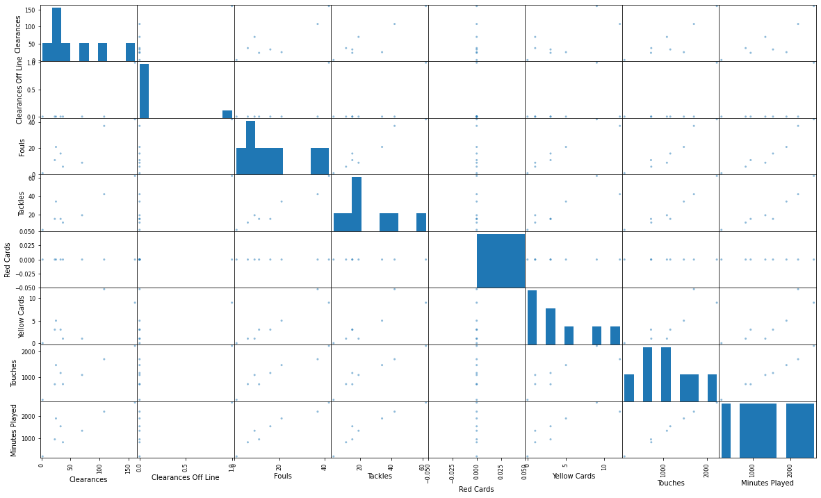
= scatter_matrix("position == 'DF'" )['Clearances' ,'Clearances Off Line' ,'Fouls' ,'Tackles' ,'Red Cards' ,'Yellow Cards' ,'Touches' ,'Minutes Played' ]= (20 ,12 ))
There are some:
bad choices (clearances off the line - only a couple of players have at least 1);not so obvious but not interesting - the more you play the more your KPI is;
potentially distinguishable KPIs.
What would be the best way to put it on the graph?
Scaling
If we want to create player profiles, we cannot just say Cech made X saves while Leno made Y. We need to normalise it. The most precise would be to do it by minutes played. So tackles per minute played or passes per minute played .
Having these numbers, we can already iterate to find the best representation.
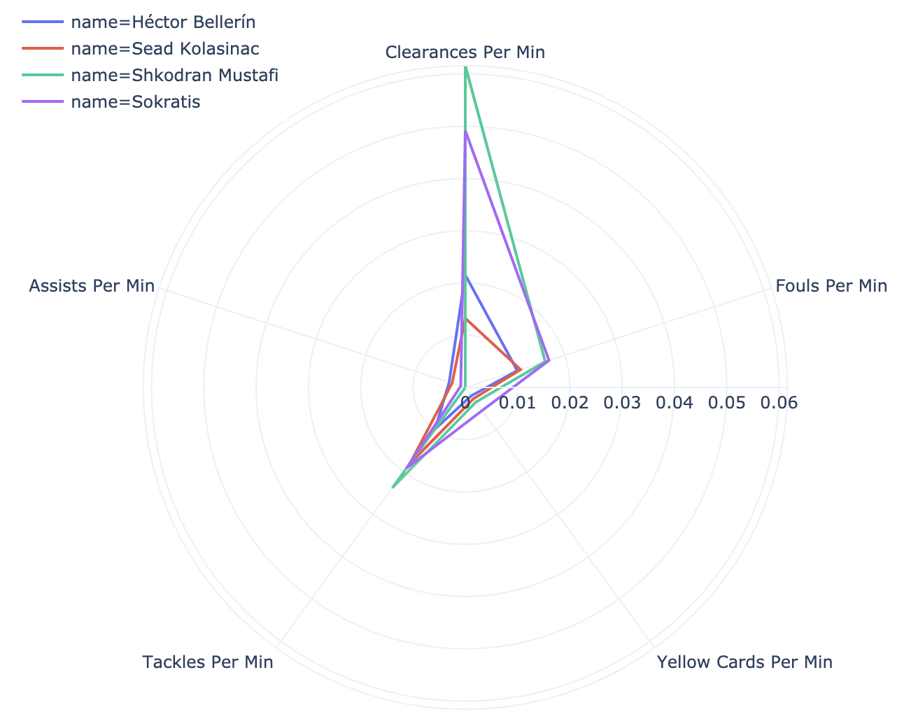
Ratios as-is
The good part here - the real values are displayed for the KPIs. We can see Mustafi is completing around 0.06 clearances per minute played, more than anyone else. The problem - it’s hard to have all the numbers at the same scale, so some metrics skew the scale towards one direction and so it becomes hard to see values for smaller values.
Mustafi - first in memes but also completing around 0.06 clearances and 0.025 tackles per minute, more than any other defender in a team.
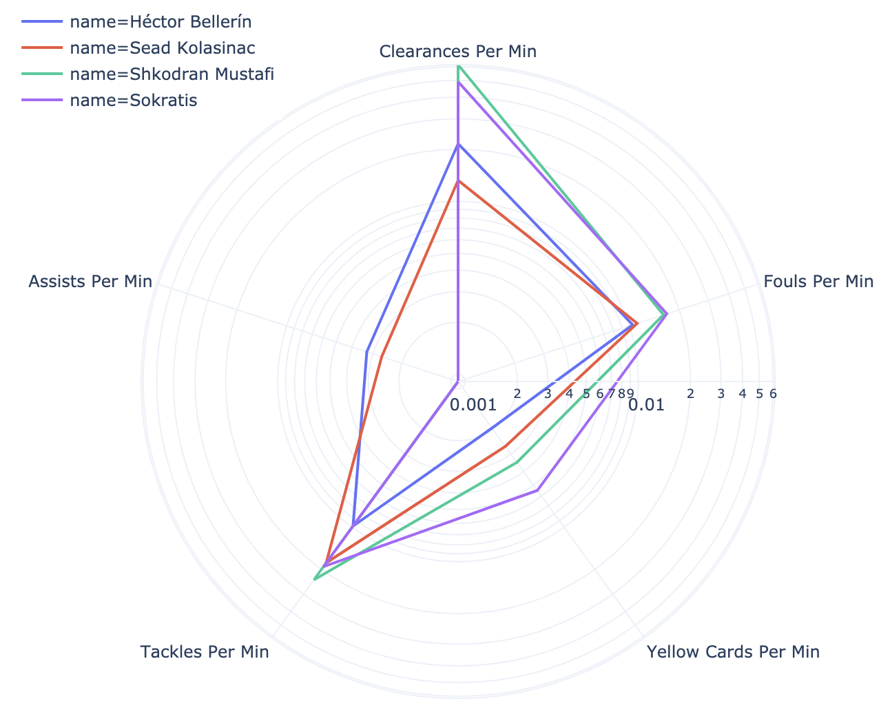
Log-scaling
We can try to play with axis scales to get a more equal distribution of numbers. As you can see now graphs are more equally distributed, but it’s a mess in readability.
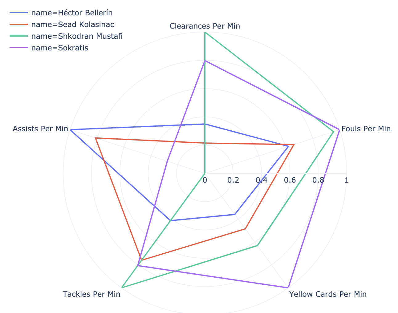
Relative scaling
We can divide values by the maximum for the metric at this position. So all players will get a percentage from the maximum for the position in a team. As for the example above: Mustafi will get 1 for the clearances, Sokratis around 0.8 from that and so on.
Personally, I like the last approach most, even though with it we are losing the interpretability.
Figure 1: Different attempts at a radar chart
By Position
Goalkeepers
Code
= training.query("position == 'GK'" )['high_claim_per_appearance' , 'punches_per_appearance' , 'saves_per_appearance' 'passes_per_appearance' ,'clearances_per_appearance' , 'Minutes Played' ]= {'high_claim_per_appearance' :'High Claims' , 'punches_per_appearance' : 'Punches' , 'saves_per_appearance' :'Saves' , 'passes_per_appearance' : 'Passes' ,'clearances_per_appearance' : 'Clearances' })= gk.max ().to_dict()= pd.DataFrame(gk.unstack()).reset_index()= ['kpi' , 'name' , 'value' ]'denom' ] = gk.kpi.map (max_map)'value' ] = gk.value / gk.denom
kpi
High Claims
High Claims
Punches
Punches
Saves
Saves
Passes
Passes
Clearances
Clearances
Minutes Played
Minutes Played
name
Bernd Leno
Petr Cech
Bernd Leno
Petr Cech
Bernd Leno
Petr Cech
Bernd Leno
Petr Cech
Bernd Leno
Petr Cech
Bernd Leno
Petr Cech
value
0.364583
1.0
1.0
0.571429
0.820312
1.0
0.900391
1.0
1.0
1.0
1.0
0.206349
denom
0.857143
0.857143
0.5
0.5
4.0
4.0
32.0
32.0
1.0
1.0
2835.0
2835.0
Code
= px.line_polar(gk, r= 'value' , theta= 'kpi' , line_dash= 'name' , color= 'name' , line_close= True = "plotly_white" , width= 800 )= 'lines' , line_width= 5 )= dict (x= 0.7 , y= 1.1 ))
Cech was getting around 20% of playing time compared to Leno.
Distinctive styles : Cech is doing much more high claims while Leno uses more punches.
Cech has a better “saves per minute” ratio, but also - might be the result of him playing much less.
4 most played Defenders
Code
= training.query("position == 'DF' and Appearances > 18" )['clearances_per_min_played' , 'fouls_per_min_played' , 'yc_per_min_played' 'tackles_per_min_played' ,'passes_per_min_played' , 'Minutes Played' , 'assists_per_min_played' ]= {'clearances_per_min_played' : 'Clearances' , 'fouls_per_min_played' : 'Fouls' 'yc_per_min_played' : 'Yellow Cards' ,'tackles_per_min_played' : 'Tackles' 'passes_per_min_played' : 'Passes' , 'assists_per_min_played' :'Assists' })= df.max ().to_dict()= pd.DataFrame(df.unstack()).reset_index()= ['kpi' , 'name' , 'value' ]'denom' ] = df.kpi.map (max_map)'value' ] = df.value / df.denom
kpi
Clearances
Clearances
Clearances
Clearances
Fouls
Fouls
Fouls
Fouls
Yellow Cards
Yellow Cards
Yellow Cards
Yellow Cards
Tackles
Tackles
Tackles
Tackles
Passes
Passes
Passes
Passes
Minutes Played
Minutes Played
Minutes Played
Minutes Played
Assists
Assists
Assists
Assists
name
Héctor Bellerín
Sead Kolasinac
Shkodran Mustafi
Sokratis
Héctor Bellerín
Sead Kolasinac
Shkodran Mustafi
Sokratis
Héctor Bellerín
Sead Kolasinac
Shkodran Mustafi
Sokratis
Héctor Bellerín
Sead Kolasinac
Shkodran Mustafi
Sokratis
Héctor Bellerín
Sead Kolasinac
Shkodran Mustafi
Sokratis
Héctor Bellerín
Sead Kolasinac
Shkodran Mustafi
Sokratis
Héctor Bellerín
Sead Kolasinac
Shkodran Mustafi
Sokratis
value
0.349637
0.214844
1.0
0.797709
0.620299
0.66036
0.954555
1.0
0.358611
0.484788
0.630688
1.0
0.412695
0.758747
1.0
0.805571
0.758673
0.761175
1.0
0.934498
0.586233
0.722753
1.0
0.840918
1.0
0.811111
0.0
0.278854
denom
0.061568
0.061568
0.061568
0.061568
0.016826
0.016826
0.016826
0.016826
0.005457
0.005457
0.005457
0.005457
0.023709
0.023709
0.023709
0.023709
0.674952
0.674952
0.674952
0.674952
2615.0
2615.0
2615.0
2615.0
0.003262
0.003262
0.003262
0.003262
Code
= px.line_polar(df, r= 'value' , theta= 'kpi' = 'name' , line_dash= 'name' , line_close= True , template= "plotly_white" )= 'lines' , line_width= 4 )= dict (x= 0 , y= 1.1 ))
Mustafi leads on most defensive metrics. He also played most minutes from all defenders (3rd overall, after Leno and Aubameyang).
Sokratis has a similar profile, with the exception that he leads by far in yellow cards.
Bellerin and Kolasinac have more offensive profiles , both taking third place in overall team assists rank (5 each, Bellerin played less).
Midfielders
Code
= training.query("position == 'MF' and Appearances > 20" )['assists_per_min_played' , 'dispossessed_per_min_played' 'goals_per_min_played' ,'passes_per_min_played' ,'shots_per_min_played' , 'tackles_per_min_played' 'touches_per_min_played' , 'Minutes Played' ]= {'assists_per_min_played' :'Assists' , 'dispossessed_per_min_played' :'Dispossessed' 'goals_per_min_played' :'Goals' ,'passes_per_min_played' :'Passes' ,'shots_per_min_played' :'Shots' 'tackles_per_min_played' :'Tackles' ,'touches_per_min_played' :'Touches' })= mf.max ().to_dict()= pd.DataFrame(mf.unstack()).reset_index()= ['kpi' , 'name' , 'value' ]'denom' ] = mf.kpi.map (max_map)'value' ] = mf.value / mf.denom
kpi
Assists
Assists
Assists
Assists
Assists
Assists
Assists
Dispossessed
Dispossessed
Dispossessed
Dispossessed
Dispossessed
Dispossessed
Dispossessed
Goals
Goals
Goals
Goals
Goals
Goals
Goals
Passes
Passes
Passes
Passes
Passes
Passes
Passes
Shots
Shots
Shots
Shots
Shots
Shots
Shots
Tackles
Tackles
Tackles
Tackles
Tackles
Tackles
Tackles
Touches
Touches
Touches
Touches
Touches
Touches
Touches
Minutes Played
Minutes Played
Minutes Played
Minutes Played
Minutes Played
Minutes Played
Minutes Played
name
Aaron Ramsey
Granit Xhaka
Henrikh Mkhitaryan
Lucas Torreira
Matteo Guendouzi
Mesut Özil
Nacho Monreal
Aaron Ramsey
Granit Xhaka
Henrikh Mkhitaryan
Lucas Torreira
Matteo Guendouzi
Mesut Özil
Nacho Monreal
Aaron Ramsey
Granit Xhaka
Henrikh Mkhitaryan
Lucas Torreira
Matteo Guendouzi
Mesut Özil
Nacho Monreal
Aaron Ramsey
Granit Xhaka
Henrikh Mkhitaryan
Lucas Torreira
Matteo Guendouzi
Mesut Özil
Nacho Monreal
Aaron Ramsey
Granit Xhaka
Henrikh Mkhitaryan
Lucas Torreira
Matteo Guendouzi
Mesut Özil
Nacho Monreal
Aaron Ramsey
Granit Xhaka
Henrikh Mkhitaryan
Lucas Torreira
Matteo Guendouzi
Mesut Özil
Nacho Monreal
Aaron Ramsey
Granit Xhaka
Henrikh Mkhitaryan
Lucas Torreira
Matteo Guendouzi
Mesut Özil
Nacho Monreal
Aaron Ramsey
Granit Xhaka
Henrikh Mkhitaryan
Lucas Torreira
Matteo Guendouzi
Mesut Özil
Nacho Monreal
value
1.0
0.176996
0.538524
0.186073
0.0
0.25426
0.356797
1.0
0.334326
0.74795
0.578892
0.71183
0.960538
0.079288
0.825301
0.438225
1.0
0.230349
0.0
0.786904
0.147233
0.648453
1.0
0.539397
0.744561
0.831103
0.715386
0.699188
0.833723
0.389036
1.0
0.352575
0.250615
0.211982
0.126199
0.937048
0.760976
0.623358
1.0
0.751821
0.252269
0.68834
0.696084
1.0
0.654089
0.776378
0.824114
0.714137
0.762703
0.530988
1.0
0.657337
0.95122
0.856457
0.696122
0.744102
denom
0.004518
0.004518
0.004518
0.004518
0.004518
0.004518
0.004518
0.020331
0.020331
0.020331
0.020331
0.020331
0.020331
0.020331
0.00365
0.00365
0.00365
0.00365
0.00365
0.00365
0.00365
0.897641
0.897641
0.897641
0.897641
0.897641
0.897641
0.897641
0.029805
0.029805
0.029805
0.029805
0.029805
0.029805
0.029805
0.027322
0.027322
0.027322
0.027322
0.027322
0.027322
0.027322
1.113155
1.113155
1.113155
1.113155
1.113155
1.113155
1.113155
2501.0
2501.0
2501.0
2501.0
2501.0
2501.0
2501.0
Code
= px.line_polar(mf, r= 'value' , theta= 'kpi' , color= 'name' , line_dash= 'name' ,= True , template= "plotly_white" ,= 800 ) # , color_discrete_sequence= px.colors.sequential.Plasma[-3::-1]) = 'lines' , line_width= 5 )= dict (x= 1 , y= 1.1 ))
There are two clear patterns on the chart: defensive and offensive . Xhaka and Torreira are representatives of the former, while Mkhitaryan and Özil of the latter.
Ramsey is an interesting exception of a “complete” midfielder here, leading by assists per minute played, but also participating a lot in tackles.
Forwards
Code
= training.query("position == 'FW' and Appearances > 10" )['assists_per_min_played' , 'missed_chances_per_min_played' , 'goals_per_min_played' 'offsides_per_min_played' , 'shots_per_min_played' , 'dispossessed_per_min_played' 'fouls_per_min_played' ]= {'assists_per_min_played' :'Assists' , 'missed_chances_per_min_played' :'Missed Chances' 'goals_per_min_played' :'Goals' , 'offsides_per_min_played' : 'Offsides' 'shots_per_min_played' :'Shots' , 'dispossessed_per_min_played' :'Dispossessed' 'fouls_per_min_played' :'Fouls' })= fw.max ().to_dict()= pd.DataFrame(fw.unstack()).reset_index()= ['kpi' , 'name' , 'value' ]'denom' ] = fw.kpi.map (max_map)'value' ] = fw.value / fw.denom
kpi
Assists
Assists
Assists
Missed Chances
Missed Chances
Missed Chances
Goals
Goals
Goals
Offsides
Offsides
Offsides
Shots
Shots
Shots
Dispossessed
Dispossessed
Dispossessed
Fouls
Fouls
Fouls
name
Alex Iwobi
Alexandre Lacazette
Pierre-Emerick Aubameyang
Alex Iwobi
Alexandre Lacazette
Pierre-Emerick Aubameyang
Alex Iwobi
Alexandre Lacazette
Pierre-Emerick Aubameyang
Alex Iwobi
Alexandre Lacazette
Pierre-Emerick Aubameyang
Alex Iwobi
Alexandre Lacazette
Pierre-Emerick Aubameyang
Alex Iwobi
Alexandre Lacazette
Pierre-Emerick Aubameyang
Alex Iwobi
Alexandre Lacazette
Pierre-Emerick Aubameyang
value
0.952713
1.0
0.573279
0.180638
0.616211
1.0
0.188848
0.644221
1.0
0.105857
1.0
0.879028
0.51565
0.939445
1.0
1.0
0.857514
0.425511
0.19926
1.0
0.233808
denom
0.003194
0.003194
0.003194
0.008422
0.008422
0.008422
0.008056
0.008056
0.008056
0.009581
0.009581
0.009581
0.03442
0.03442
0.03442
0.028398
0.028398
0.028398
0.020359
0.020359
0.020359
Code
= px.line_polar(fw, r= 'value' , theta= 'kpi' , color= 'name' , line_dash= 'name' ,= True , template= "plotly_white" ,= 800 , text= 'value' )= 'lines' , line_width= 5 )= dict (x= .8 , y= 1.1 ))
Lacazette and Aubameyang are 2nd and 4th in most minutes played during the season.
Lacazette fouls five times more than Aubameyang or Iwobi.
Aubameyang leads on goal effectiveness, while Iwobi and Lacazette are great in assists .
Final thoughts
I used canva to assemble the graphs above into the final image , added some red-white colours. I didn’t come up with any breakthroughs, of course. But I had a couple of interesting observations and discoveries during the process. And had some fun too!
The greatest benefit was to document the process itself. As Jason Fried urges people to write more to really think the idea through, just sitting down and writing the process of analysis was rewarding.